Computer Vision Part 1: Loading Images with Python🔗
Intro to Loading Images with OpenCV and Matplotlib in a Python Notebook (+ Bonus using PIL / Pillow)
1. Import and inline setup🔗
At the start of our notebook we put %matplotlib inline, this isn't necessary in normal python because there is no inline viewing.
We import matplotlib.pyplot as plt for ease of typing.
We also import opencv (cv2) to load images. Matplotlib uses Numpy arrays (ndarray) to display, so does opencv.
Later we'll using PIL / Pillow to load images, which will require converting to numpy anyway
Use ctrl + enter to run cells more easily, or use the play button above or to the left of cells.
Once we've run both of the following cells we'll be able to view images. If this fails then your virtual environment probably doesn't have both matplotlib and cv2 installed, so you'll need to pip install... or conda install... based on your setup.
Also note that PIL has inline image viewing, I'm not sure if it's supported in all notebooks. There's also HTML5 viewing.
OpenCV docs for version 3.4.2 (Relatively similar between versions 2.x and 4.x, the different pip and conda and conda-forge sources will give different verisions)
| Python | |
|---|---|
| Python | |
|---|---|
| Text Only | |
|---|---|
1 2 | |
2. Fetching some image files🔗
In this step we do a basic folder / directory search with glob.glob, which is a lot like ls in the terminal. I'll use a String to specify the directory and an asteriks *.png to indicate a wildcard (i.e. it selects any filename that ends in '.png' in the directory. (We have to import it to use it, but it's built into python)
Where your files are may vary, in this case I use a relative path ('./start_images') since the file.ipynb is in the same folder as my data folder. You could also use an absolute path ('/Users/username/datasets/mycooldata')
Reference for glob Reference for directories
| Python | |
|---|---|
| Python | |
|---|---|
| Text Only | |
|---|---|
1 2 3 4 5 | |
3. Use OpenCV to Load image files into numpy ndarrays🔗
Now that we have the file paths that tell where each image is, we can load them.
We'll make an empty list that we'll append with loaded images. We 'Image Read' (imread) in the images and specify OpenCV to give us a 3-channel image (Red, Green, Blue), which is what we generally want to work with (This is included because if you want to use a texture / sprite with empty alpha you should use cv2.IMREAD_UNCHANGED to load in a 4-channel image with alpha transparency).
OpenCV (and by extension Numpy in most cases) follows the order of (ROWS, COLUMNS, CHANNELS) for the array shape. So when we use the .shape attribute on an OpenCV image we get a 3-tuple of (Height, Width, Channels). If it is 1-channel it will be a 2-tuple of (Height, Width) If working in PIL see 9.
You can do this with as many files as you want, but if you try to load too many your computer may slow down / python will Out Of Memory error.
If you have an image in the same folder a non-absolute path will probably work: "myimage.png", "./myimage.png"
Reference for OpenCV non-notebook
| Python | |
|---|---|
| Text Only | |
|---|---|
1 | |
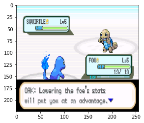
4. Dislpay a single Image using Matplotlib🔗
At this point you've got all the images loaded and ready to display, now it's just up to you whether you to spread out the calls or make a grid with matplotlib
If we use more than one plt.imshow() call in the same cell one will not actually get displayed (there may be a workaround to this, we'll use a grid at step 6). You can try commenting out the second plt.imshow() call, you should get a different image when you run it again.
| Python | |
|---|---|
| Text Only | |
|---|---|
1 | |
5. OpenCV Color Caveat🔗
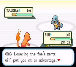
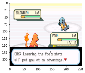
OpenCV loads images in B-G-R order (Blue, Green, Red), as opposed to R-G-B which I'm prety sure most of the rest of the world uses (Except people really into color, who use HSV or HSL or whatever)
What this implies: - We could swap the first and last channel to display it as RGB easily with matplotlib. - When saving a file OpenCV assumes the image is in BGR.
We'll focus on the first implication for now and discuss the second when we use PIL / Pillow.
We use OpenCV's cvtColor ('Convert Color') in the following way: recolored_image = cv2.cvtColor(original_image, cv2.TYPE_OF_CONVERSION).
Conversions you'll probably use the most:
- cv2.COLOR_BGR2RGB: convert BGR to RGB (essentially the same as cv2.COLOR_RGB2BGR, swaps first and third channel)
- cv2.COLOR_BGR2GRAY: convert BGR to Grayscale (1-channel) (RGB2GRAY also available)
- cv2.COLOR_GRAY2BGR: convert Grayscale to BGR 3-channel (GRAY2RGB also available)
Reference for changing colors (Bonus Object Tracking demo using HSV color space)
| Python | |
|---|---|
| Text Only | |
|---|---|
1 | |

6. Displaying multiple Images with Matplotlib🔗
Now our RGB images can display nicely, so let's move on to displaying multiple images in a grid with matplotlib.
We'll use matplotlib subplots(), but you can find many implementations of 'make grid of images' with matplotlibt using other functions
Reference for matplotlib subplots (also see figures keywords link)
HTML colornames that are valid for matplotlib
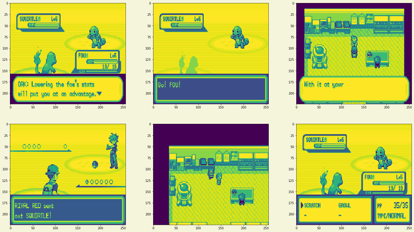
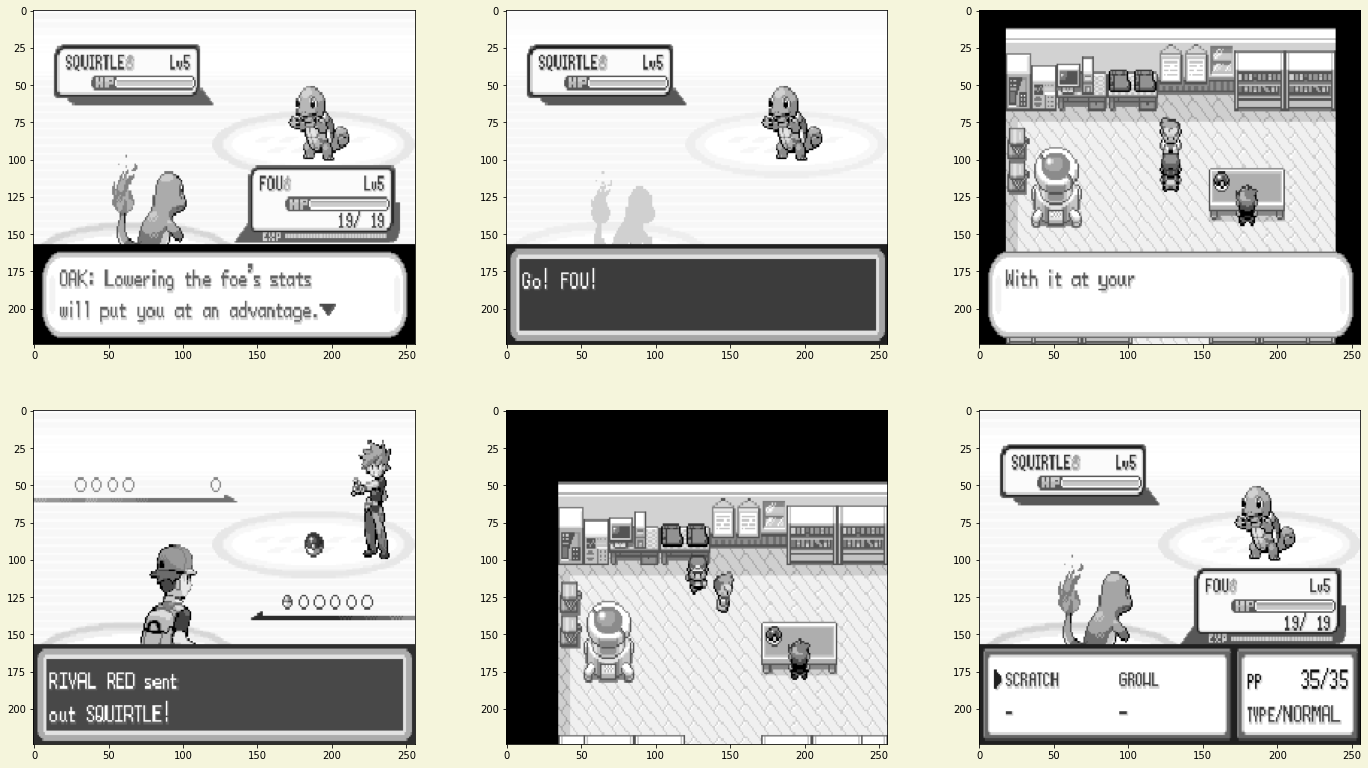
7. Matplotlib Grayscale Color Caveat🔗
Well we've run into another display issue. Our grayscale images are 1 channel, but why does matplotlib show these colors? Grayscale / 1-channel images can be used in many domains, and matplotlib isn't just for plotting images, so their default colormap from values to colors is not Grayscale, but instead it's something called viridis and used to be jet. (I dont' know anything about the uses of these, but there's a whole talk on why they make viridis, so there's theory behind it).
We'll just make sure to specify to matplotlib that we want to use the gray colormap whenever we imshow an image. Or use another one of matplotlib colormaps.
We also will treat this as a whole new figure (a new set of subplots), so we'll use the plt.subplots() call again
Reference for default map in matplotlib
| Python | |
|---|---|
Bonuses!🔗
Those are the most important points about using Python Glob to get files, OpenCV to load, MatplotLib to display.
We'll now go into more specific use cases - Plotting image changes on multiple images in a grid - Using PIL / Pillow and the differences with OpenCV - Saving Images
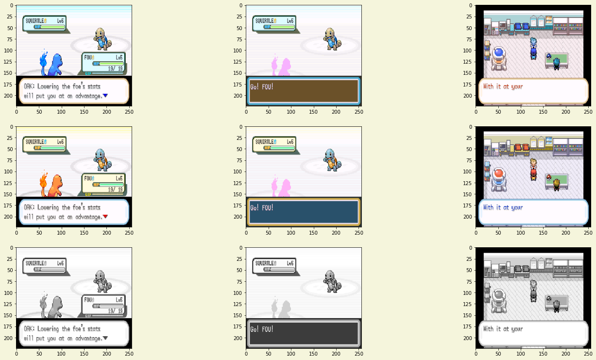
8. Function for plotting image changes on multiple images in a grid🔗
Commonly when we do image processing tasks we'll have an input, perform some operation (often using a mask or another image), and then have some output image that's different from the original. Maybe we want to perform multiple operations and view all of them, then we'd have an extra_output for each input
We usually want to compare the output with the input to make sure our operation is doing what we want, and we usually want to ensure it's working on multiple images.
What this implies:
- If we maintain a list of inputs and a list of outputs that correspond to each input we can display each input in one row, and each output on the next to compare
- If inputs and outputs have a one-to-one relationship, it'll be simple to go through both in one list but display in multiple rows
- We can treat any transformation or step of our program as an operation, and might want to check that each one works as we're intending
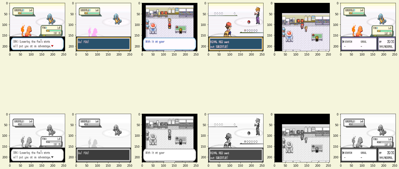
We'll make a function that takes a list of ALL the image lists concatenated and the number of inputs (length of our inputs list) to display each list row by row.
Note: The only error checking we do is for single channel image vs RGB(A), so the list best be divisible by the number of samples🔗
(We'll also only use 3 images for size constraints)
| Text Only | |
|---|---|
1 2 | |
9a. Using PIL / Pillow Image library🔗
PIL / Pillow / Python Imaging Library is also super popular, but the images are in a different format than OpenCV and can't be displayed immediately by Matplotlib, so we'll go over some of the differences. I'll make notes in the code that show where to be careful when dealing with Pillow vs OpenCV.
Installing this library has changed over the years. Using pip install Pillow should get you the correct version. Alternatively, the pytorch extension torchvision has Pillow as a dependency, so if you pip install torchvision you should get a working Pillow.
I'll mostly only refer to the Image Module (Documentation), ImageColor and ImageChops may also be relevant to your tasks.
We'll also need direct access to Numpy for conversions and displaying, we import as np for ease of typing
NOTE Older guides on PIL import it differently. You probably want to use from PIL import Image🔗
| Python | |
|---|---|
| Text Only | |
|---|---|
1 2 | |
9b. Loading Images with PIL🔗
Not much different from OpenCV, just a different command
| Text Only | |
|---|---|
1 2 | |
9c. Display PIL images in matplotlib🔗
One way to compare with OpenCV images is using matplotlib, but we need to convert. So we'll use the numpy conversion asarray() to get something matplotlib can use.
As you should see, PIL loads images in RGB format by default.
| Python | |
|---|---|
| Text Only | |
|---|---|
1 2 3 4 5 6 7 | |
9d. Convert PIL image colors🔗
This is a good time to talk about in-place vs out-of-place operations. In-Place means something affects the object directly, and thus will have some effect on the object. Out of Place means the original object isn't altered during the operation and a brand new object is returned by the function.
Most operations we're using here are Out of Place, so be sure to save the result in a new variable assignment (as in gray_pil = pil_image.convert()) or append the result to a list.
But be on the look out for In-Place operations, especially in Numpy. They use less memory because they don't save two copies of the thing you're working with, but they'll affect your original data, so side effect bugs may occur in your program.
For displaying, we'll convert to numpy pre-emptively
See Pillow image modes for some more info
- "1" is 1-bit pixels, black or white
- "L" is 8-bit black and white (0...255 scale)
- "RGB" is 8-bit RGB
10a. Saving your images🔗
After a long hard day of image processing and converting, you probably want to save the results so that your computer doesn't have to do all that hard work all over again.
NOTE The middle image that displays correctly is actually backwards to OpenCV
We'll use a directory that is at the same level as our .ipynb in our filesystem, so we can reach it with ./out_images as opposed to a full absolute path (ex. /home/username/projects/segmentation/outputs)
| Text Only | |
|---|---|
1 2 3 | |

| Text Only | |
|---|---|
1 | |
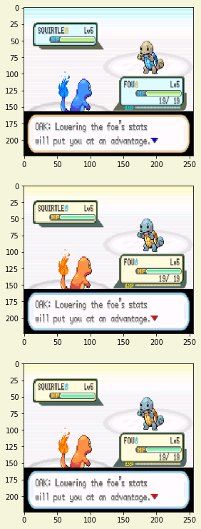
10b. Saving Colors Correctly🔗
Again, OpenCV uses BGR by default on save and load, PIL uses RGB. If you converted to RGB with OpenCV you should convert color back before you save.
So when we saved the OpenCV BGR Image loaded_w_cv.png it saved as a png that will be read as RGB (except by OpenCV).
When we saved the PIL RGB Image loaded_w_pil.png it also saved as a png that will be read as RGB (except by OpenCV)
To demonstrate, we'll load all 3 with PIL again, since that defaults to RGB loading
| Text Only | |
|---|---|
1 2 3 | |
11. Wrap-up🔗
Those are all the basic loading, converting, and saving operations that I've needed to use with OpenCV and PIL, working in an ipython notebook or in regular .py scripts
As a final code snippet, we'll go from OpenCV Image (numpy ndarray) to PIL Image, as we haven't actually needed to do that without saving first. You'd use this if you want to pass numpy loaded arrays into a PIL-based image processing pipeline (ex. torchvision transforms)
NOTE Again check your color conversions. Image.fromarray() expects an array in RGB form and will treat whatever 3-channel array you give it as such.
| Text Only | |
|---|---|
1 2 3 | |
Created: June 7, 2023