Time Series Data Part 4: A Full Stack Use Case🔗
Roommate Spending Ledger Visualization🔗
![]()
Using Pandas + Plotly + SQLite to show a full stack use case of Time Series Data.
Analyze spending over time per person (could be adapted to categories / tags / etc).
See: Github Repo
Idea🔗
One time series that any financially independent person should pay attention to is their spending over time.
Tracking your spending gets complicated with roommates and budgets for different categories. It also complicates your understanding of your data with a glance, which is where charts and graphs can help.
There are many personal budgeting and even group budgeting apps, but I wanted to make the simplest possible and stick to the Data and Visualizations as an MVP.
One way to get this data is from a CSV export from a bank account or credit card company. In Part 3 is an app that uses this method on general time series data. Upload a CSV with some column for time stamps and some column to forecast and tune your own prediction model!
The main drawbacks to this paradigm:
- Can't share data between people / sessions
- Can't persist data
- Can't incrementally add data
- Can't update data
Another way is the CRUD paradigm explored in my Streamlit Full Stack Post. With this method we'll be able to operate on individual data points and let our friends / roommates add to it!
(Of course the CSV paradigm could be blended with this)
Now for each aspect of the app, from Backend to Front
DevOps🔗
There's not much real DataOps in this project since the data is self-contained.
That said, there are some DevOps aspects that are important in the time series world:
- Deployment: having a webserver accessible to multiple users
- Integration: how to get updated code into the deployment(s)
Leaning on Streamlit Cloud sharing checks both of these boxes with ease.
By including a requirements.txt and specifying a python version for the image, we get a free CI/CD pipeline from any push to a github branch (more providers to come).
It'll provide us with an Ubuntu-like container that installs all requirements and tries to perform streamlit run streamlit_app.py, yielding a live webserver accessible to the public for public repos!
Backend🔗
The Data Engineering aspect involves a bit of data design and a bit of service writing.
I decided the minimum data to track expenses are:
purchased_date- The day on which the purchase was made
purchased_by- The name of the person who made the purchase
price_in_cents- Price of the purchase. Tracked in cents to avoid floating point perils
Relying on SQLite, we'll have to represent the date as a string, but pandas will help us transform it to a date / datetime object.
A table creation routine with SQLite for this might look like:
| Text Only | |
|---|---|
1 2 3 | |
We also get a free autoincrementing rowid from SQLite, which will differentiate any purchases by the same person on the same day for the same amount!
Python Object Model🔗
That's all well and good for a DBA, but what about the Python glue?
Using pydantic / dataclasses is my preferred way to make Python classes that represent database objects or API responses.
Splitting the Model into a child class for the internal application usage and parent class for database syncing is one way to handle auto-created id's and optional vs. required arguments.
| Python | |
|---|---|
| Text Only | |
|---|---|
1 | |
Seeding🔗
To get some values for playing around with and demonstrating Create / Update, here's a snippet of seeding the database
| Text Only | |
|---|---|
1 | |
200 times we'll create and save an Expense object with a hardcoded id and some random values for date, purchaser, and price. (Note the randomized days max out at 28 to avoid headaches with february being short. There's probably a builtin to help with random days, maybe just timedelta with random amount is easier)
Using kwarg placeholders of the form :keyname lets us pass the dictionary / JSON representation of our Python object instead of specifying each invidual field in the correct order.
The rest of the CRUD operations follow a similar pattern. Reading is the only hacky function to allow filtering / querying at database level before pulling ALL records into memory.
Reshaping the Data🔗
The Data Science aspect of this involves massaging the data into something useful to display.
The data as it stands is not actually the well formed time series you might have thought.
Sure the date stamps are all real, but what value do we read from them?
The goal is to track spending (price_in_cents in the database).
But what if we have multiple purchases on the same day? Then we might start treating all the purchases on a given day as stochastic samples and that is not our use case. (But that might fit your use case if you are trying to model behaviour based off of many people's purchases)
Enter the Pandas🔗
Utilizing Pydantic to parse / validate our database data then dumping as a list of dictionaries for Pandas to handle gets us a dataframe with all the expenses we want to see.
Passing a start_date, end_date, and selections will limit the data to certain time range and purchased_by users.
| Python | |
|---|---|
| price_in_cents | purchased_date | purchased_by | rowid | |
|---|---|---|---|---|
| 0 | 9662 | 2022-12-13 | Alice | 2 |
| 1 | 9925 | 2022-12-12 | Alice | 138 |
| 2 | 6287 | 2022-12-10 | Bob | 92 |
For this analysis I mainly care about total purchase amount per day per person. This means the rowid doesn't really matter to me as a unique identifier, so let's drop it.
(This indexing selection will also re-order your columns if you do or do not want that)
| purchased_date | purchased_by | price_in_cents | |
|---|---|---|---|
| 0 | 2022-12-13 | Alice | 9662 |
| 1 | 2022-12-12 | Alice | 9925 |
| 2 | 2022-12-10 | Bob | 6287 |
To handle the summation of each person's purchase per day, pandas pivot_table provides us the grouping and sum in one function call.
This will get us roughly columnar shaped data for each person
| Python | |
|---|---|
| price_in_cents | |||
|---|---|---|---|
| purchased_by | Alice | Bob | Chuck |
| purchased_date | |||
| 2020-01-01 | 0 | 0 | 1566 |
| 2020-01-20 | 0 | 7072 | 0 |
| 2020-01-26 | 0 | 0 | 9982 |
Looking more like a time series!
pivot_table had the minor side effect of adding a multi index, which can be popped off if not relevant
| purchased_by | Alice | Bob | Chuck |
|---|---|---|---|
| purchased_date | |||
| 2020-01-01 | 0 | 0 | 1566 |
| 2020-01-20 | 0 | 7072 | 0 |
| 2020-01-26 | 0 | 0 | 9982 |
Side note:
I also added a feature where "All" is a valid selection in addition to all purchased_by users.
The "All" spending per day is the sum of each row!
(We can sanity check this by checking for rows with 2 non-zero values and sum those up to check the All column)
| purchased_by | Alice | Bob | Chuck | All |
|---|---|---|---|---|
| purchased_date | ||||
| 2020-08-12 | 3716 | 5896 | 0 | 9612 |
| 2020-10-09 | 4881 | 2595 | 0 | 7476 |
| 2021-04-11 | 3965 | 3623 | 0 | 7588 |
| 2021-10-19 | 3332 | 627 | 611 | 4570 |
| 2022-01-08 | 5021 | 11061 | 0 | 16082 |
| 2022-03-01 | 6895 | 4857 | 0 | 11752 |
| 2022-08-03 | 8642 | 258 | 0 | 8900 |
| 2022-09-11 | 4751 | 1617 | 0 | 6368 |
To fill in date gaps (make the time series have a well defined period of one day), one way is to build your own range of dates and then reindex the time series dataframe with the full range of dates.
Grabbing the min and max of the current index gets the start and end points for the range. Filling with 0 is fine by me since there were no purchases on those days
| Python | |
|---|---|
| purchased_by | Alice | Bob | Chuck | All |
|---|---|---|---|---|
| purchased_date | ||||
| 2020-01-01 | 0 | 0 | 1566 | 1566 |
| 2020-01-02 | 0 | 0 | 0 | 0 |
| 2020-01-03 | 0 | 0 | 0 | 0 |
To get the cumulative spend up to each point in time, pandas provides cumsum()
| purchased_by | Alice | Bob | Chuck | All |
|---|---|---|---|---|
| purchased_date | ||||
| 2020-01-01 | 0 | 0 | 1566 | 1566 |
| 2020-01-02 | 0 | 0 | 1566 | 1566 |
| 2020-01-03 | 0 | 0 | 1566 | 1566 |
| 2020-01-04 | 0 | 0 | 1566 | 1566 |
| 2020-01-05 | 0 | 0 | 1566 | 1566 |
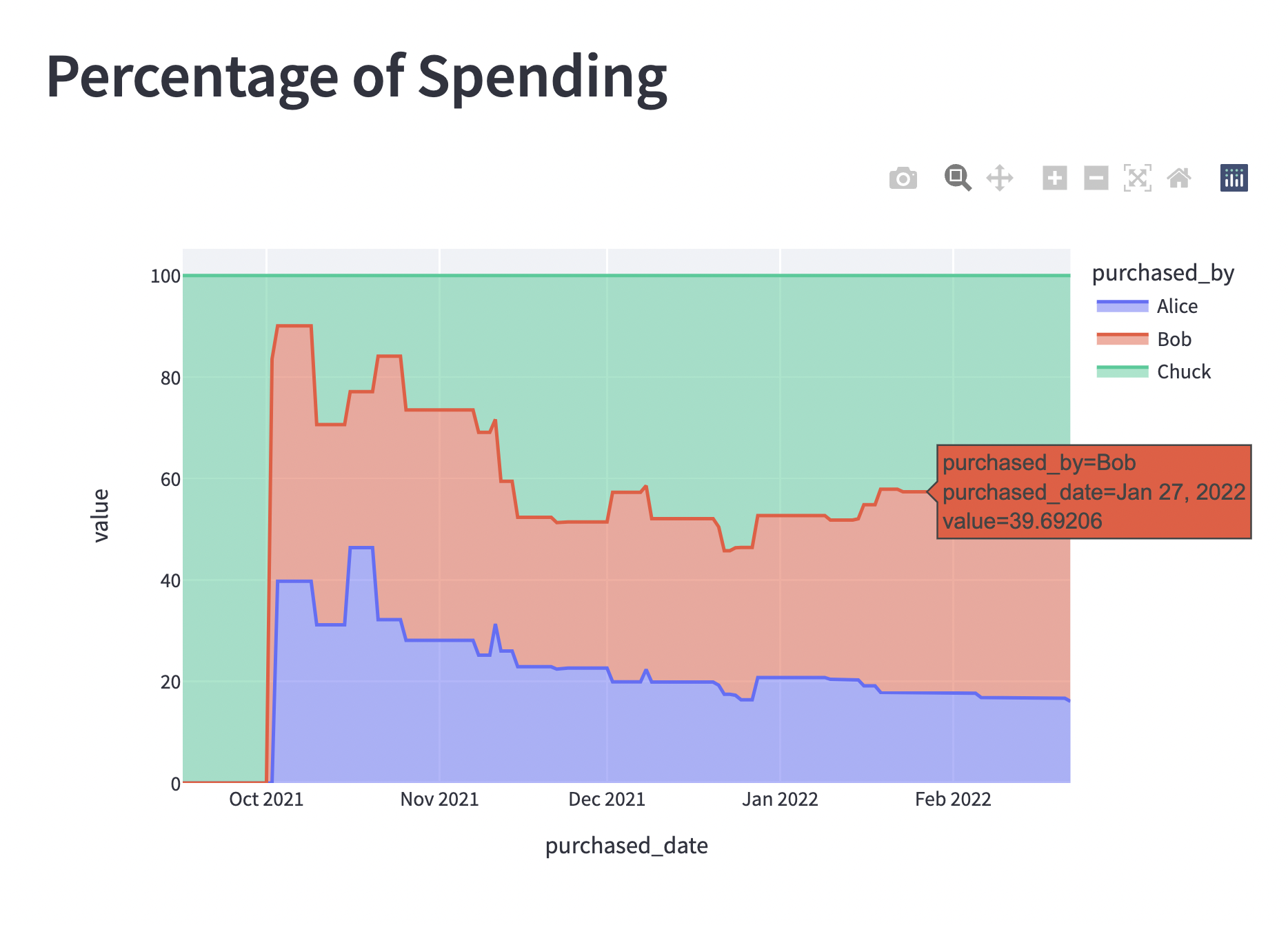
And to analyze percentage contributed to the whole group's cumulative spending we can divide by the sum of each cumulative row.
(We included the "All" summation already, so this case is actually slightly over-complicated)
| Python | |
|---|---|
| purchased_by | Alice | Bob | Chuck |
|---|---|---|---|
| purchased_date | |||
| 2020-01-01 | 0.0 | 0.0 | 50.0 |
| 2020-01-02 | 0.0 | 0.0 | 50.0 |
| 2020-01-03 | 0.0 | 0.0 | 50.0 |
| 2020-01-04 | 0.0 | 0.0 | 50.0 |
| 2020-01-05 | 0.0 | 0.0 | 50.0 |
Grabbing the totals of each spender might be a nice metric to display.
This could also be grabbed from the end of the cumulative data
| Python | |
|---|---|
| purchased_by | value | |
|---|---|---|
| 0 | Alice | 3565.16 |
| 1 | Bob | 3019.81 |
| 2 | Chuck | 3826.65 |
| 3 | All | 10411.62 |
Pandas also provides a convenient rolling() function for applying tranformations on moving windows.
In this case let's get the cumulative spending per 7 days per person.
Notice that the value will stay the same on days when the person made $0.00 of purchases, since x + 0 = x!
| purchased_by | Alice | Bob | Chuck | All |
|---|---|---|---|---|
| purchased_date | ||||
| 2020-01-01 | 0.0 | 0.0 | 1566.0 | 1566.0 |
| 2020-01-02 | 0.0 | 0.0 | 1566.0 | 1566.0 |
| 2020-01-03 | 0.0 | 0.0 | 1566.0 | 1566.0 |
| 2020-01-04 | 0.0 | 0.0 | 1566.0 | 1566.0 |
| 2020-01-05 | 0.0 | 0.0 | 1566.0 | 1566.0 |
| 2020-01-06 | 0.0 | 0.0 | 1566.0 | 1566.0 |
| 2020-01-07 | 0.0 | 0.0 | 1566.0 | 1566.0 |
| 2020-01-08 | 0.0 | 0.0 | 0.0 | 0.0 |
We don't have to sum the rolling values though. Here we grab the biggest purchase each person made over each 30 day window.
Notice that a given value will stick around for up to 30 days, but will get replaced if a bigger purchase occurs!
| purchased_by | Alice | Bob | Chuck | All |
|---|---|---|---|---|
| purchased_date | ||||
| 2020-01-01 | 0.0 | 0.0 | 1566.0 | 1566.0 |
| 2020-01-02 | 0.0 | 0.0 | 1566.0 | 1566.0 |
| 2020-01-03 | 0.0 | 0.0 | 1566.0 | 1566.0 |
| 2020-01-04 | 0.0 | 0.0 | 1566.0 | 1566.0 |
| 2020-01-05 | 0.0 | 0.0 | 1566.0 | 1566.0 |
| 2020-01-06 | 0.0 | 0.0 | 1566.0 | 1566.0 |
| 2020-01-07 | 0.0 | 0.0 | 1566.0 | 1566.0 |
| 2020-01-08 | 0.0 | 0.0 | 1566.0 | 1566.0 |
| 2020-01-09 | 0.0 | 0.0 | 1566.0 | 1566.0 |
| 2020-01-10 | 0.0 | 0.0 | 1566.0 | 1566.0 |
| 2020-01-11 | 0.0 | 0.0 | 1566.0 | 1566.0 |
| 2020-01-12 | 0.0 | 0.0 | 1566.0 | 1566.0 |
| 2020-01-13 | 0.0 | 0.0 | 1566.0 | 1566.0 |
| 2020-01-14 | 0.0 | 0.0 | 1566.0 | 1566.0 |
| 2020-01-15 | 0.0 | 0.0 | 1566.0 | 1566.0 |
| 2020-01-16 | 0.0 | 0.0 | 1566.0 | 1566.0 |
| 2020-01-17 | 0.0 | 0.0 | 1566.0 | 1566.0 |
| 2020-01-18 | 0.0 | 0.0 | 1566.0 | 1566.0 |
| 2020-01-19 | 0.0 | 0.0 | 1566.0 | 1566.0 |
| 2020-01-20 | 0.0 | 7072.0 | 1566.0 | 7072.0 |
| 2020-01-21 | 0.0 | 7072.0 | 1566.0 | 7072.0 |
| 2020-01-22 | 0.0 | 7072.0 | 1566.0 | 7072.0 |
| 2020-01-23 | 0.0 | 7072.0 | 1566.0 | 7072.0 |
| 2020-01-24 | 0.0 | 7072.0 | 1566.0 | 7072.0 |
| 2020-01-25 | 0.0 | 7072.0 | 1566.0 | 7072.0 |
| 2020-01-26 | 0.0 | 7072.0 | 9982.0 | 9982.0 |
| 2020-01-27 | 0.0 | 7072.0 | 9982.0 | 9982.0 |
| 2020-01-28 | 0.0 | 7072.0 | 9982.0 | 9982.0 |
| 2020-01-29 | 0.0 | 7072.0 | 9982.0 | 9982.0 |
| 2020-01-30 | 0.0 | 7072.0 | 9982.0 | 9982.0 |
| 2020-01-31 | 0.0 | 7072.0 | 9982.0 | 9982.0 |
Now Make it Pretty🔗
Since we did most of the work in pandas already to shape the data, the Data Analysis of it should be more straightforward
We'll use a helper function to do one final transformation that applies to almost all our datasets
| Python | |
|---|---|
| purchased_date | purchased_by | value | |
|---|---|---|---|
| 0 | 2020-01-01 | Alice | 0.00 |
| 1 | 2020-01-02 | Alice | 0.00 |
| 2 | 2020-01-03 | Alice | 0.00 |
| 3 | 2020-01-04 | Alice | 0.00 |
| 4 | 2020-01-05 | Alice | 0.00 |
| ... | ... | ... | ... |
| 4307 | 2022-12-09 | All | 10152.88 |
| 4308 | 2022-12-10 | All | 10215.75 |
| 4309 | 2022-12-11 | All | 10215.75 |
| 4310 | 2022-12-12 | All | 10315.00 |
| 4311 | 2022-12-13 | All | 10411.62 |
4312 rows × 3 columns
Seems like it's undoing a lot of work we've already done, but this Long Format is generally easier for plotting software to work with.
In this case we keep purchased_date as a column (not index), get a value column called value, and a column we can use for trend highlighting which is purchased_by
After that, plotly express provides the easiest (but not most performant) visualizations in my experience
| Python | |
|---|---|
For more of the plotting and charting, check it out live on streamlit!
Created: June 7, 2023